

meta data for this page
Drive Analog Characteristics
The Analog Characteristic test is used to perform an analysis of the analog electronics and signal filtering that takes place within your floppy drive. Reading it takes a fair bit of knowledge about how a floppy drive functions at a low level, but it is still possible for a novice to glean the essential bits of the test in order to make sure that their drive is functioning properly or is suitable for imaging a particular disk format.
A floppy drive is an analog device and not a digital one. It reads an analog signal from the floppy disk and sends a pulse every time it sees the signal change. (The floppy drive controller has the job of turning those pulses into digital bits.) Various drive models used various combinations of read amplifiers, filtering, and a good smattering of assumptions about the incoming signal in order to send pulses at the appropriate time, These components help the drive determine if a signal is happening “too fast” and should be ignored, or “too slow” and we should turn up the amplifier because it must be missing some data.
Many computer systems used pretty similar ways of storing data to a disk, like FM or MFM encoding, and similar media types, like double density or high density. The encoding defines rules for how flux transitions should be organized on disk to represent data. The media type allows for differing densities or rates of flux transitions. Many drive manufacturers focused on only one of these encoding standards and therefore when we ask a drive to read some other form of encoding, it can potentially run into issues doing so.
What do all these graphs mean?
The test screen is comprised of 3 separate graphs:
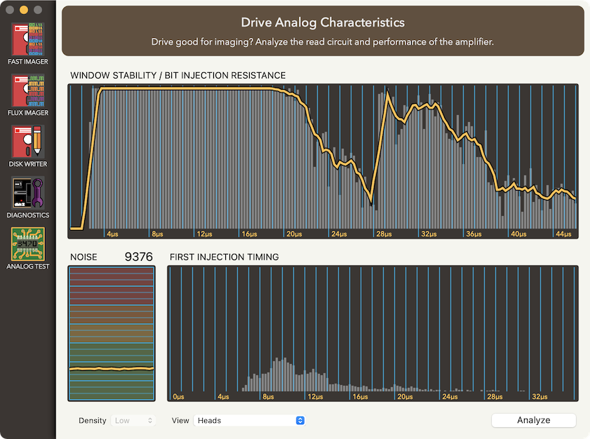
Noise
The Noise test in the lower left gives us a baseline for the density of noise that is generated by the drive when in “full panic” mode. Having a high noise level here doesn't mean that a drive is bad or will have trouble reading a disk. It is more the representation of the worst-case scenario of a drive trying to read a disk when it cannot find any data. Many drives have an automatic gain control function that tries to increase the sensitivity of the read head in order to lock in on the flux transitions on the disk. Unfortunately, the sensitivity can be turned up so much that the drive starts making up data that doesn't actually exist. The graph shows the number of “fake” transitions that the drive sends per rotation on a track that has been wiped of data.
Window Stability
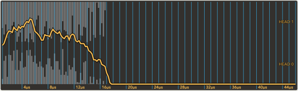
The Window Stability graph at the top of the window is the analysis of what the drive can and cannot process reliably. The gray vertical lines show the results for individual tests at various flux frequencies long lines are high success rate, and short or no line means lower success rate. The gold line in the graph is a breakdown of the signal reliability along with factoring in things like spindle motor speed fluctuations and such. The most important thing you need to recognize in this graph is the durations which are covered with the gold line pinned to the top which is 100% reliability. The above graph shows that the signal is 100% stable from 3.75µs through to 19µs. If you aren't familiar with how data is stored on disks at a very low level, then that range of stability probably means absolutely nothing to you. And as an expert in this, I could give you the definitive answer of “well, it depends on what kind of disks you want to be imaging”. Here is a quick table of some popular disk formats:
| Media | Encoding | Platform | 100% Stability Required |
|---|---|---|---|
| 5.25 DD | MFM | 360K PC | 4µs - 8µs |
| 5.25 HD | MFM | 1.2M PC | 2µs - 4µs |
| 5.25 DD | Apple GCR | 143K Apple II | 4µs - 12µs (up to 16µs recommended) |
| 5.25 DD | Commodore GCR | 170K C64 | 3.25µs - 12µs |
| 5.25 HD | Victor 9000 GCR | 612K | 1.25µs - 7.5µs |
| 3.5 DD | MFM | 720K PC | 4µs - 8µs |
| 3.5 HD | MFM | 1.44M PC | 2µs - 4µs |
| 3.5 DD | Apple GCR | 800K Mac (in PC drive) | 2.5µs - 12.0µs |
The screen shot above shows the stability of a 5.25 DD drive. In looking at the table above, the drive is capable of reading all of the 5.25 DD formats except for the Commodore GCR. The C64 requires stability down to 3.25µs, but this drive is only stable down to 3.75µs. And indeed when using this drive to image C64 disks, there are many errors in the first half of disks.
First Injection Timing
The First Injection Timing graph is a bit more complex to explain and for the most part is irrelevant to most users. If you really want to know, there is some details about what it is showing in the last section of this page.
Test settings
There are only 2 settings for the analog test. The first setting is the Density. This allows you to specify Low (DD) or High (HD) density. Be sure to use the proper media type with each setting or you will not get accurate results. For PC drives that support low and high density operation, many used different sets of filters for each density. The screen shots below show the same drive set to different densities with low on the left, and high on the right. The gold line clearly shows that the characteristics of the drive are quite different for each density.
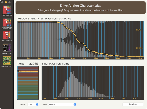
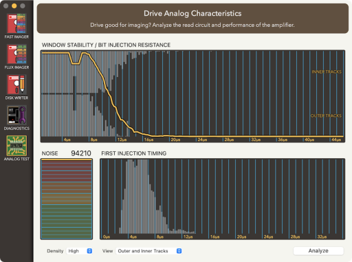
The second setting is View. This allows you to perform the tests slightly differently. The Heads option puts the head in the center of the disk and performs analysis on each head (in a 2 headed drive). The bottom drive head (head 0) will be shown on the bottom half of the graph, and the top head (head 1) will be shown on the top half. The Outer and Inner Tracks will perform the test with the head at each end of the media. The physical spacing of fluxes differs on the outer vs inner tracks, and so this lets you see how different the drive deals with each end.
If the Noise test is a worst-case scenario, why do we care about it?
For the most part when reading normally structured unprotected disks, you won't care about the noise level at all. Where it comes into play tends to be with various forms of copy protection that use no-flux areas on the disk (spiral track protections and such). These kinds of areas are common for Apple II games. The below image shows three disk renderings of the same disk rendered in drives with low, medium, and high levels of noise.
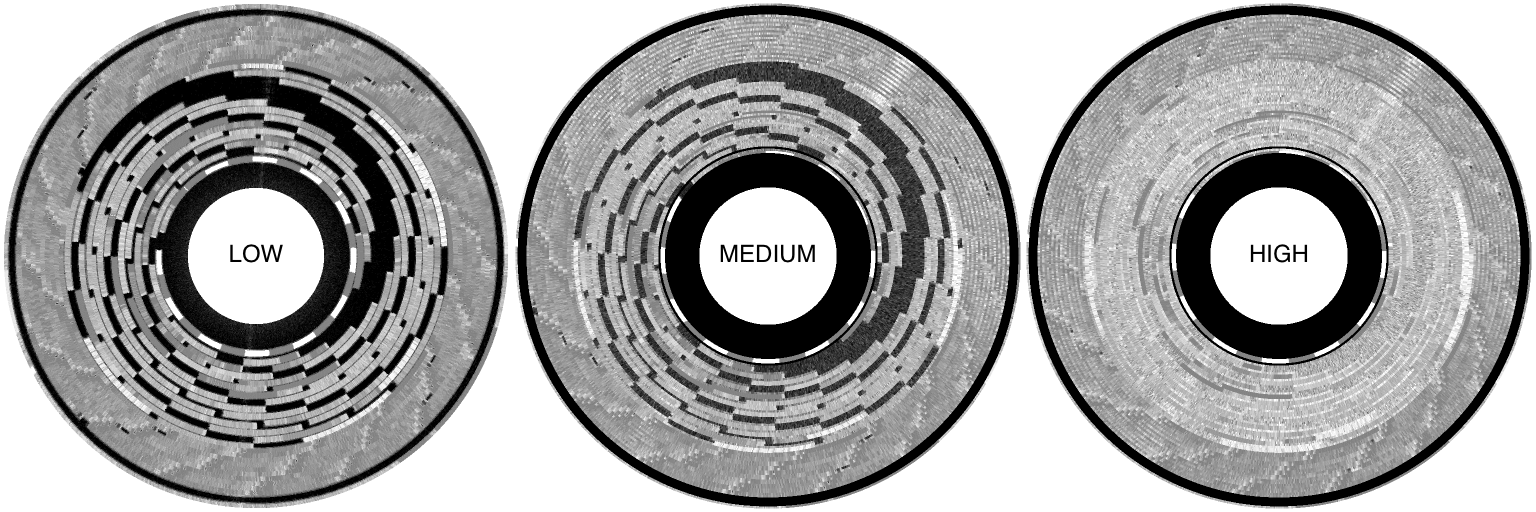
The black areas shown are have no flux transitions written in them. The low noise is the most accurate representation of the disk, whereas the high noise is completely unrecognizable as being the same disk. The real data on the disk is likely intact just fine, but with high levels of noise it becomes almost impossible for the disk analyzer to be able to tell what is real data and what is fake. When it comes to disks that are structured like this, it is definitely best to have a drive that is as quiet as possible. Just for reference: the Low drive was an Apple Disk II, the Medium drive was a Panasonic JU-475-3, and the High was a TEAC FD-55GFR.
My graph doesn't look anything like that.
If your graph looks like below (or worse) with no 100% stability, then the first thing to do is try to clean your drive head(s). There can also be an issue with the floppy disk you are testing with, such as physically shedding the media surface or the incorrect density. If cleaning heads and changing disks doesn't resolve the issue, it is possible that there is an issue with the drive itself.
How exactly does this work?
The primary analog test uses a test track that is comprised of a whole bunch of smaller tests. A test has a header, gap, payload, and settle field. The header contains information about the specific test (like the gap size). Following that is the gap (no flux area) whose duration ranges from 1µs to 48µs in 250ns increments. Then there is a payload which is a special bit sequence that is used to be able to detect bit slip, desynchronization, and other conditions. And then the settle which is a bit pattern that lets the analog amplifier/gain control/whatever cool down before the next test.
To create the test track, the track is wiped (WRREQ on to engage head erase coil and writing no data), then the tests are generated and written.
The test track is then read 50-ish times. What the test is checking for is the integrity of the gap and payload. If the gap is clean (no bits injected) and the payload is as well, then that is a success and it adds to the gray lines in the Stability graph. In the case of a failure, the payload is checked for integrity and if the payload is intact, then we check the gap. If the gap has a spurious transition (injected bit), then the time offset from the last flux transition of the header to the first spurious transition is recorded onto the First Injection Timing graph at the bottom.